
Level 2
 The Level 2 record keeping resource has been designed to build upon the record keeping modules covered in Level 1. The record keeping and benchmarking modules are designed to be used by a wide range of producers and management systems. Some operations may not fit perfectly into one level for all of the topics. For example, your financial record keeping may already be at the intermediate or advanced level, but you may feel that you are more of a beginner in the forage and grassland area. Each of the levels have been developed to target a level of experience where level 1 is a good starting point for beginners; level 2 is for someone that is more than a beginner but not quite advanced; and level 3 is designed to be the most advanced level. Your current record keeping practices may be a combination of levels depending on topic, which is normal and to be expected!
On this Page
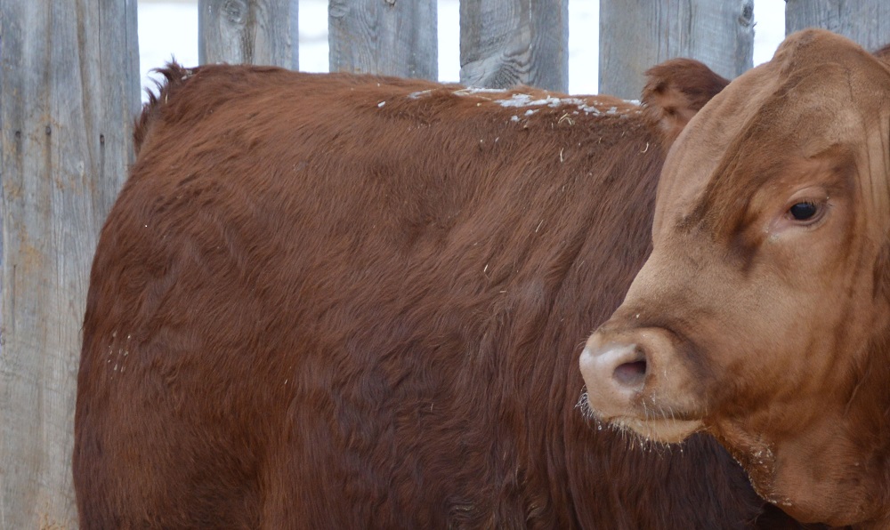
Animal Health and Performance
Animal health and performance records can be useful for making management decisions. Keeping track of your health treatments and performance indicators throughout the year can be useful information to have when evaluating your production goals. Having readily accessible records can also be handy when marketing cattle to prospective buyers.
Body Condition Scores
|
Industry Benchmark BCS of 3.0 |
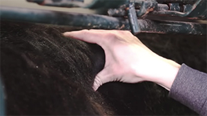
Cows with an ideal body condition score (3.0 on a scale of 1-5) rebreed up to 30 days sooner than thin cows, which allows more cows to calve in the first 21-day cycle. This can add up to 42 lbs in calf weaning weight since the calves born earlier in the calving season will be heavier at weaning time. Cows in ideal body condition also have pregnancy rates double those of cows in poor condition, have improved milk production, passive immunity transfer, fewer cases of abortion and stillbirth, healthier calves, and fewer instances of calving problems.
The salvage value of cull cows in good condition is also higher. Very thin cows are more likely to experience negative outcomes during transport or to be condemned at harvest. Thin cows reflect poorly on producers and the industry.
To learn how to do a hands on assessment of body condition scoring visit our BCS page.
Data to record: Body condition score (1-5) of each animal or sub-sampling from larger group.
When to record it: One of the best times to body condition score is during fall processing or when pregnancy checking. This will give you time to add condition on thinner cows before winter sets in.
 Example: At fall processing in October a sample of 30 cows from the larger group of 150 cows was evaluated for BCS. The average BCS for the 30 cows assessed was 2. The summer months had been particularly dry resulting in reduced forage availability and thinner cows. A decision was made to feed test the stored forages to ensure the cow herd would have adequate nutrition during the winter months to reach a BCS of 3 before breeding. Before releasing the cow herd back onto pasture for breeding BCS will be assessed again.
Trade-offs: increasing body condition scores will require additional investment for feed, but this may be offset by an improved reproductive rate for the following season.
Example goal:
- Improve body condition scores of the mature cow herd to 3 before the next breeding season.
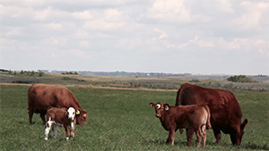
Calving Distribution
|
Industry Benchmark 60% of calves born in the first 21 days |
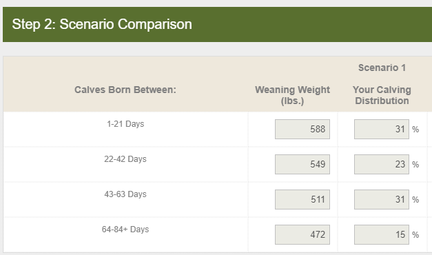
Establishing and maintaining breeding momentum is important. Once a cow is bred in the first part of the breeding season, she has a greater likelihood of breeding back early in the years to follow. Cows that are bred early will have calves that have greater potential to gain by weaning time, resulting in a uniform calf crop and improved profitability. For example, a calf born in the first cycle compared to one born twenty-one days later will have the potential to gain an extra 39 lb (i.e. 1.85 lb/day for 21 days) more than its later-born counterpart. This can result in additional revenue of $81 per calf if sale price is $2.08/lb.
The standard industry target is to have at least 60% of females calving within the first cycle, followed by 25% calving between 21-42 days, 10% between 42-63 days and the remaining 5% calving in the fourth and final cycle. An ideal distribution could be 70-20-10 with a condensed breeding season of three cycles (63 days). The value of calving distribution calculator can help you determine your distribution using your own data.
Data to record: Bull turn out dates, breeding dates (AI, or observed natural breeding), birth dates
When to record it: Record the bull turn out date(s) or breeding dates if using AI. Record calving dates at calving.
Example: In Level 1 we used the example of a herd of 65 females, with the calving period starting with the first calf born on January 2, 2019. The very last calf was born on April 10, 2019. To determine the length of the calving period, count the number of days between January 2 and April 10. This equals a 99-day calving period.
Using the calving distribution calculator, it was determined that 31% of calves were born in the first cycle. There may be several factors impacting the distribution besides cow fertility. This can include body condition of the cow herd, cow to bull ratio, bull performance, weather, illness, or management factors such as when the bulls were pulled.
In order to reduce calving period length, you would first need to identify the factors contributing to the longer calving period before culling cows calving outside 84 days to ensure this is not just a cow fertility issue.
Trade offs: Depending on your management system you may require two calving periods. A front-loaded calving period can require extra labour costs due to a greater workload to pick up bulls at the end of the breeding season.
Shortening the calving period can result in more open cows as later-calving females won’t have a chance to rebreed. This can result in short term losses from fewer calves sold at weaning.
Producers that utilize community pastures or even rent grass away from home may not be in control of when bulls are removed or have facilities to pick up bulls in 63 or 84 days.
Example goals:
- Reduce calving period length to less than 84 days within two years
- Reduce calving period to less than 63 days by year five
- Have 60% of calves born in the first 21 days by year five
Cow-to-bull ratio (cow:bull)
|
Industry Benchmark 25 cows: 1 bull |
The capacity of the bull to perform during breeding is also limited by the fertility of the cowherd. Therefore, most efforts are placed upon ensuring that reproductive potential of the females in the herd is optimized. We often assume that the bull will do his job, if we make the correct management decisions regarding the cow herd.
The economic implications of failure or reduced performance of bulls in a natural mating program can result in major losses. Even with the correct managerial and financial investments in place to ensure that the cow herd is reproductively competent, if reproductive failure occurs as a result of bull management, a tremendous loss in terms of reproductive efficiency is likely.
The more females that a bull can breed in a given season, the more optimal or efficient is the use of the capital invested in that sire. However, if you increase the cow:bull ratio, the likelihood increases that the bull’s mating capacity will be exceeded and fertility during the breeding season will be reduced. There is a point of diminishing returns, in terms of the reproductive efficiency of your herd and uniformity of the calf crop, if the mating capacity of the bull is exceeded.
The number of bulls required for effective reproductive efficiency will depend on the age of the bull, size of the pasture, topography, length of the breeding season and condition of the bull. A shorter breeding season will not only improve weaning weights but will also give the bull time to rest.
Data to record: Number of cows per bull
When to record it: Record at bull turn out date(s)
Example: Using the same example from above, the 65 cows were kept on pasture with the same bull from June until October, a 65:1 ratio. To improve the calving distribution for the next year, the length of the breeding season was reduced, and an additional bull was purchased which changed the ratio to 33:1.
Trade offs: Underestimating the performance of your bulls resulting in an investment of additional bulls that were not needed.
If multiple bulls are used in a pasture this can result in fighting versus breeding. The impact depends on age of bulls, number of watering holes and pasture topography.
Example goals:
- Purchase additional bull(s) to service more groups of cows effectively
Mature Cow Weight
|
Industry Benchmark 45% of cow weight |
Recording mature cow weights aims to “right size” cows for the productivity of the environment. Smaller cows do well in low productivity environments and can wean calves weighing 45% or more of their body weight. Very productive environments can support heavier cows that also wean 45% of their body weight. An apparent trend towards a smaller cow size is partly due to wanting the right size cow for the environment in semi-arid climates. But there are also advantages to larger cows in high productivity environments.
Data to record: Weights of cows
When to record it: During processing in the spring and fall
To determine the weaning weight as a percentage of cow weight simply divide the average weaning weight by the average cow weight and multiply by 100.
| Average Pounds Weaned ÷ Average Mature Cow Weight X 100 = Weaning weight as percentage of cow weight |
Example: For 110 females exposed, their average weight was 1215 lbs:
593 lbs average weaning weight ÷ 1215 lbs average cow weight x 100 = 49%
Trade offs: selecting for larger mature weights may result in greater feed costs.
Example goals:
- Match a significant percentage of cow weight and forage intake to forage production prior to the next breeding season
Calculating pounds weaned per cow exposed
| Pounds Weaned per Exposed Female = (Total Pounds Weaned) ÷ (Number of Exposed Females) |
Commercial cow-calf producers generate revenue based on total pounds of calf weaned and sold. There are only two ways to increase total pounds of calf weaned and that is by increasing the size of each calf weaned or by increasing the number of calves weaned. Pounds of calf weaned per cow exposed combines the herd reproductive rate, calf death loss, and genetics for growth and maternal traits into one number.
Data to record: Weaning weights, number of exposed females
When to record it: Record weaning weights at weaning and record number of females exposed prior to bull turnout.
Example: In Level 1 we calculated that the group of 105 calves had a total weaning weight of 65,205 lbs, an average of 621 lbs per calf weaned. If we were to include the number of females that were exposed at the beginning of the breeding season things may look a bit different. Assuming a herd of 110 cows:
65,205 lbs total pounds weaned ÷ 110 females exposed = 593 lbs per exposed female
If the number of exposed females was actually 120 females this would change to:
65,205 lbs average weaning weight ÷ 120 females exposed = 543 lbs per exposed female
Example goals:
- Improve reproductive efficiency by 2% within two years
- Reduce calf death loss between birth and weaning to 4% with four years
Forage and Grasslands
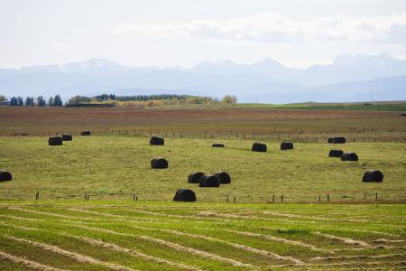
 Winter Feed and Stored Forages
Cow body condition in late fall or early winter has a major impact on the total amount and quality of feed required. Cows in thin condition in the fall must gain weight throughout the winter to be able to deliver a live healthy calf, provide adequate amounts of milk, become pregnant and produce a calf the following year.
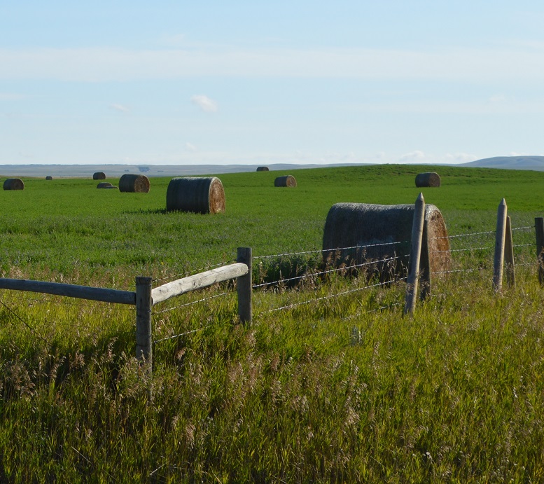
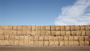
Across Canada many beef cows are fed a significant amount of conserved forage during winter. While extending the grazing season with stockpiled grass and annual forage crops can reduce the length of the feeding season on many operations, there is still a lot of baling and chopping done in preparation for the colder months. Harvesting, storing and delivering the herd's winter rations are the largest variable cost of production. Even small improvements in the system can result in significant savings.
Benchmarks
Comparing benchmarks for forage production is a challenge due to the variability from location to location. Comparing production numbers within your own operation is one way to manage your year to year production and to determine whether your management decisions are having the desired effect on production. Having a baseline of your typical production can also aid when making decisions during atypical years. For example, how you can manage in a drought year versus a bumper crop year.
Crop Records
When managing forages, just like other crops, the implementation of good record-keeping is valuable for managing plant productivity, crop rotations, and soil fertility.
Complete and accurate records help demonstrate your protection of soil, water and other environmental resources and will help you analyze the performance of your farm’s forage production system.
Table 1: Example Crop Record
| Field ID/ Location | Acreage/Hectares | Number of bales/ loads | Weight of bales/loads | Inputs | Yield |
| Old Farm | 100 acres | 150 | 1470 lbs | Manure, 3 loads, October 2018 | 1 tonne/acre |
| Old Farm | 100 acres | 150 | 1544 lbs | None | 1.01 tonne/acre |
Field identification
Keeping an accurate description of the location of each field will assist with keeping precise production records.
Data to record: Legal land location, identification recognized by land managers/staff, size in acres or hectares
When to record it: At time of purchase, after dividing a field
Field inputs
Research has indicated that fertilization can bring the productivity of a stand back to its original level without the expense of re-seeding. However, even when fertilizer is applied at recommended rates, the target yields may not be achieved, making it a risky proposition. The goal of fertilizing is to decrease the per unit cost of production. Higher yields do not necessarily translate into lower costs or increased profits. Only when the value of the additional production surpasses the cost of application does it reduce the per unit cost of production and increase margins. The profitability of fertilizing forage crops is highly variable and depends on timely rains, the cost of the fertilizer and hay prices. As these factors change, so will the feasibility of fertilizing.
If an assessment of the current forage stand shows that there is a sufficient quantity of the desired plant species still present, then fertilization can be an effective tool to rejuvenate and increase forage yields. By applying nutrients that are limiting, as determined by taking a soil test, forage production can be improved.
A soil test is essential to determine which nutrients are currently available and which may be deficient. Without this critical information there is a good chance that your investment may be money misspent. Knowing what nutrients to apply and in what quantity is an important first step in a fertility program.
Data to record: Treatment, date, volume, location
When to record it: Following application
Yields
Examining profit margins per field can be easily calculated when hay yield and price per ton are recorded. Producers need to know yields and market prices in order to estimate potential profitability - or calculate actual net returns after the hay is marketed or for own use. A greater awareness of your yields could direct you to making changes that will bring about greater productivity and profitability from a given field.
Data to record: Weight of bales, number and weight of cart loads
When to record it: At harvest
Yield calculation:
A 100-acre field produced 150, 5’x5’ round bales that each weighed 1470 lbs (667 kg). Dry matter was not yet tested.
Yield = (150 bales x 1470 lbs/bale)/ (100 acres x 2205 lbs) = 1 tonne per acre
Example crop production goals:
- Improve forage yield at the Old Farm by 5% within one year, pending adequate weather conditions
Feed Inventory
 After all of the effort and expense of producing the forage, ensuring that it is being efficiently utilized by the animals is the critical last step. Developing a feed inventory is the first step to help track feed utilization and thus improve feed management.
Efficient feed utilization includes:
- Matching the quality of the forages to the right animal group
- Monitoring feed disappearance
- Minimizing feed wastage
- Comparing the amount of feed offered to what the cows should be consuming
Some things to consider:
- Current feed inventory for all types of storage units/feed types (bunkers, agbags, baleage, dry hay, bins). Calculate silage capacity in bunkers and silos here.
- Determine your feed needs by determining the number of animals and their stage of production (lactating cows, heifers, backgrounders, bulls)
- Determine potential growth. Do you plan to buy or sell any large groups?
- How much are you feeding per head per day?
- How long does this feed need to last?
- Determine the balance. Do you have enough? Can some forage be sold?
Data to record: Current inventory, number of animals and their stage of production, volume fed per day, feed test results
When to record it: February/March – allows you to make a mid-course correction prior to the next harvest season. Estimates of density will be more accurate after having fed from storage for a while, so estimates of quantity stored will be more accurate.
June/July – allows you an early warning of inadequacy of feed supplies for the up-coming feeding season. Purchases of standing crops remain an option if deficiencies are discovered.
October/November – in a drought year, when production has been unexpectedly low you may want to make a projection to see if purchased feed will be needed or if the consumption rate needs to be adjusted. This allows needed purchases when commodity prices are apt to be lower in winter and will allow purchases before December 31, assisting in tax management.
Example goals:
- Create a feed inventory after each year’s harvest and update as it is fed out
Feed Waste
The following section was adapted from Beef Cow Winter Feed Utilization page from the Ontario Ministry of Agriculture, Food and Rural Affairs.
 When producers talk about the amount they are feeding their cows, they are usually referring to the amount of forage offered and which disappears from the inventory. This will always be larger than what the cows are actually consuming. The difference is due to several factors, including:
- the wastage of forage as it is being moved from storage
- feed tramped into the ground or bedding,
- feed soiled by manure or urine,
- feed which is left uneaten until the next lot of feed is delivered,
- inedible crusts on bales which may be removed prior to feeding.
It's important to have a good idea of how feed disappearance matches up with the expected intake of the cows. If the gap is too wide, after adjusting for typical wastage, there may be some issues with the feeding system that can be corrected in order to save feed and therefore money. If actual feed intake is significantly lower than anticipated, after accounting for wastage, there may be an issue with the quality of the forage. Table 2 has some guidelines for evaluating various levels of feed disappearance.
Table 2: Interpretation of the Difference between Observed Forage Disappearance and Predicted Intake1
| % Difference2 | Interpretation |
| < 6% | Excellent utilization of forage |
| 6% to 10% | Very Good utilization; some slight improvements may be possible |
| 11% to 15% | Good utilization; some improvements possible |
| 16% to 20% | Medium utilization; significant improvements possible |
| 21% to 25% | Poor utilization; very significant improvements possible |
| >25% | Very Poor utilization; critically evaluate feeding system |
1 forages fed to beef cows under typical on farm conditions
2 (Observed disappearance - Predicted intake) / Predicted intake X 100
Here's an example of a feeding scenario:
- 50 cow management group
- Cows average 1500 lbs, in good body condition, dry, mid third of pregnancy
- Average daily temperature is -5 C°, feeding area is sheltered from the prevailing wind
- Ground conditions are dry
- Being offered 4' X 4' dry hay bales which weigh 600 lbs
- Hay was tested and is 84% DM with 54% TDN (DM basis)
Step 1: What is the expected dry matter feed intake of these cows?
| Basic cow dry matter intake calculation: | Cow dry matter intake adjusted for environment: |
| DMI = Cow wt. X % DMI (per lb of cow wt.) DMI = 1500 lbs X 2.2% Dry matter intake = 33 lbs per cow |
Adjustment for daily air temperature = 1.05 DMI = 33 lbs X 1.05 (air temp) X 1.00 (mud) |
After adjustments the expected dry matter intake per cow is 34.7 lbs.
Step 2: What is the expected actual (as fed, AF) amount of hay which would be consumed by these cows? We need to convert our estimated dry matter intake to an AF basis for the hay being offered.
| As Fed Intake calculation |
| As Fed Intake = DMI lbs / % DM in the hay AF Intake = 34.7 lbs / 84% DM AF Intake = 41.3 lbs |
So, we would expect each cow to consume about 41.3 lbs of hay per day. For the feeding group of 50 cows this would be:
| To feed 50 cows: |
| 41.3 lbs X 50 hd = 2065 lbs of hay |
Step 3: Converting this to bales of hay
2065 lbs / 600 lbs = 3.44 bales of hay per day
Step 4: The group is being fed an average of 3.5 bales per day, with a very minimal amount left in the feeders. How does this feed disappearance match up with what is expected? Let's look at it on a per head basis:
Feed disappearance/hd = 4.0 bales X 600 lbs per bale / 50 hd = 48 lbs/hd/day
Step 5: We had estimated the hay disappearance for this group in Step 2 as 41.3 lbs/hd/d. The difference between feed disappearance and estimated intake:
Difference = disappearance - estimated intake
= 48 lbs - 41.3 lbs
= 6.7 lbs
Step 6: On a percentage basis this would be:
Difference / estimated intake X 100%
6.7 lbs / 41.3 lbs X 100% = 16%
This indicates that about 16% of the feed which is being offered is not actually being eaten by the cows, there is likely significant room for improvement. It would be a good idea to closely observe the cows' feeding behavior and see how much hay is being pulled out of the feeder and lost on the ground, as well as how much forage is being left uneaten in the feeders. In trials, hay wastage when feeding round bales has been measured from 5% to 40%, with the higher range occurring when the bales are rolled out on the ground.
Data to record: Expected dry matter intake, feed disappearance
When to record it: Daily, at feeding
Example goal:
- Reduce feed waste to the 11 to 15% range using methods that reduce trampling in the next 365 days.
Feed Testing
 When you don't know the quality of feed on an operation, maintaining animal health and welfare can become significantly more difficult. Visual assessment of feedstuffs is not accurate enough to access quality and may lead to cows being underfed and losing body condition or wasting money on expensive supplements that aren't necessary.
Why should I feed test?
- Avoid subtle production problems, such as poor gains or reduced conception caused by mineral or nutrient deficiencies or excesses;
- Prevent or identify potentially devastating problems due to toxicity from mycotoxins, nitrates, sulfates, or other minerals or nutrients;
- Develop appropriate rations that meet the nutritional needs of their beef cattle;
- Identify nutritional gaps that may require supplementation;
- Economize feeding, and possibly make use of opportunities to include diverse ingredients;
- Accurately price feed for buying or selling.
One of the major benefits of feed testing is preventing costly and devastating problems before they start. Every season is different and some years there is an abundance of high-quality forage. Other years, there is a lack of available feed, or perhaps there is an abundance of low-quality forage, grain, or grain by-products available that may look economical but can potentially pose significant risks if a feed analysis has not been performed or understood. Feed testing should be completed as close as possible to when it will be fed for the most accurate results.
Learn more about the how and why of feed testing and interpreting results
Data to record: Date, type of feed sampled, volume of sample, location of sample, analysis results
When to record it: Following sampling
Example: A sample of grass silage was taken from the silage produced from the 100-acre field at the farm mentioned above. The results of the feed test were entered into the Evaluating Feed Test Results Tool on Beefresearch.ca and received the following result:
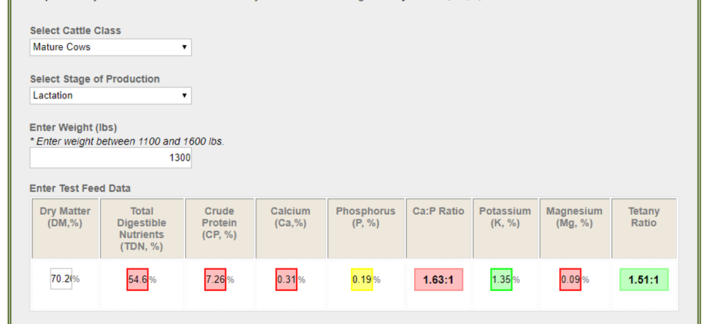
The results suggest that the feed will not be adequate to feed on its own to lactating mature cows and should be fed with additional feedstuffs such as additional energy, vitamins, minerals and a protein source. The next step will be to work with a nutritionist or ration balancing software program to determine a balanced ration for the lactating cows.
Example goals:
- Work with a nutritionist to mitigate any potential nutritional deficiencies
- Establish a location to keep all feed test results and use to monitor progress year to year
Winter Feed Ration
While hay, pasture, other forages and grains make up the largest component of livestock feed, there are many alternative feeds that can be provided and even improve the diet. Cost effective procurement of non-conventional feeds can increase profitability across the operation.
Alternative feeds can include crop residues, damaged crops, processing by-products, fruit, vegetable and bakery waste, off grade grains and even weeds. Resourceful producers will consider several factors when sourcing alternative feeds:
- cost of feed
- cost of transportation
- storage of feed including special bins, silos, or conditions to reduce spoilage
- nutritive value of feed including any deficiencies or toxicities that must be corrected
- consistency and ongoing availability of feed
- ease of integration into operation, such as special feeding management, grinding, or mixing equipment required
- palatability of feed and acceptance by livestock
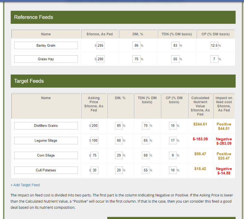
The inclusion of alternative feeds in a ration or feeding program can reduce feed costs and stretch feed supplies, while meeting nutritional requirements. Weather events such as drought, flooding, late spring frosts or hail can impact conventional feed supplies and increase prices. Many producers incorporate non-conventional feed sources into their rations to reduce costs and reliance upon hay or silage. While non-conventional feeds can be a cost-effective choice, producers will need to compare the actual costs of each feed source, along with transportation and storage to determine viability. A calculator for evaluating the relative economic value of feeds based on protein and energy content is available to assist producers when making these decisions.
Cattle require appropriate levels of energy, protein, fibre, vitamins and minerals to allow maintenance, growth, reproduction and gestation, milk production, and to support the immune system. When sourcing and adding non-conventional feeds to the ration, consult a livestock nutritionist to obtain the best advice for ration balancing. Conduct feed tests for each feed source. Balance nutrient requirements for the sex, age, body condition and stage of production of the cattle being fed. For example, straw can be a low-cost alternative feed, however, it requires supplementation with additional energy, protein and minerals to provide adequate nutrition for all classes of cattle.
Visit the alternative feeds webpage for more information about using alternative feeds and the risks and benefits of different types of feed sources.
Data to record: Type of feed, feed test results, purchase cost
When to record it: Following purchase, after feed testing
Example: Since the feed test on the grass silage was not optimal and the price of barely is higher than you would like, you decide to look into some options for alternate feeds to feed the group of lactating, mature cows. Using the Tool for Evaluating the Economic Value of Feeds Based on Nutrient Content you enter some options for feeds you are considering purchasing. The results (shown below) indicate that distillers’ grain and corn silage may be good options to supplement the herd, where the legume silage and cull potatoes may not be good options economically.
Genetics
 If you have completed the previous modules in Level 1 and 2, you may have already identified the areas of your operation where you would like to improve and have set some production goals. Once you know where you are, you can then start to plan where you would like to go. Maybe you want your calves to be heavier at weaning? Or you’re interested in more uniform coat colour, so that your calves fit into a certain market? While some of your goals will be influenced by your production practices, other goals such as higher weaning weights will be influenced by both genetic and environmental factors (nutrition, stress, health problems, weather, etc.).
Genetic change in cow-calf operations can occur both through sire selection and through replacement female selection in conjunction with cow culling.
EPDS
Expected Progeny Differences (EPDs) are estimates of an animal’s genetic merit as a parent. EPDs are the difference between the predicted average performance of an animal’s future progeny and the average progeny performance of another animal, assuming that the bulls are mated to similar cows, or vice versa. There are EPD’s across breeds but most breeds have independent EPD’s and use different measurements or units as other breeds for certain categories.
To compensate for differences in environment and management, contemporary groupings are used. Contemporary groups are animals of the same age and sex raised under the same management conditions. Once these factors are accounted for, the genetic component is the part that remains, and that is what EPDs predict.
A bull with impressive EPDs does not guarantee a superior calf crop. A common producer complaint about EPDs is that they do not seem to reflect actual data. Because EPDs rely on information provided by the producer, it is critical that the accurate information is submitted. This means reporting all performance data measured on all animals in the herd, and correctly identifying contemporary groups under different management (for example, if one group received creep feed and one group did not). In addition, billions of genetically different progeny are possible from just a single mating! There are plenty of genetic differences between full siblings. Because EPDs predict AVERAGE progeny performance, it is quite common to have a calf or two that doesn’t fit in with the rest. This is where accuracy comes in.
Accuracy is a value between 0 and 1 that reflects how close the prediction (EPD) is to the true genetic merit (breeding value) of the animal. Accuracy values increase as the amount of information known on an animal increases. Adding data on an animal’s own performance, the performance of its relatives, and performance of its progeny will increase accuracy. As accuracy gets higher, an EPD is less likely to change substantially. Some breed associations are incorporating genomic data into their EPD evaluations. By merging DNA test results with the traditional EPDs, more information can be added at a younger age, increasing the accuracy (and confidence) in that animal’s EPDs.
Although all these numbers can get confusing, selection based upon a single trait can often lead to undesired consequences. For example, selecting only for weaning weight in a production system where heifers are retained, will lead to larger mature cows, potential calving difficulties, and perhaps increased feed intake. A balanced selection approach focusing on optimizing traits for your environment and production system works much better than trying to maximize a single trait.
Heritability
Heritability is a measure of how much genetic influence there is on a particular trait. Heritability is a value between 0 and 1 and the higher the number, the more genetic influence there is on that trait. Reproductive traits tend to have low heritability rates, while weight and carcass traits are more heritable.
For example, weaning weight has a heritability of 0.24 to 0.30, which means that 24 to 30% of the differences we see in yearling weights between cattle in a herd are caused by genetics. The range of heritabilitiy shown in Table 3 has been shown as a percentage of heritability. If a trait has a low heritability, this indicates that the environment or management has a much larger influence on that trait. High heritability indicates that genetics play a relatively large role in the trait. The level of heritability in a trait will have an impact on selection decisions. Progress tends to be much slower in lowly heritable traits when attempting change through selection alone. With higher heritability, we usually can achieve more rapid progress through selection2.
Table 3: The impact of genetics or management changes on culling decisions
| Trait impacting culling decisions | Heritable/ Non-heritable | Range of heritability (%) | Improved primarily through genetics or management? |
| Cow traits | |||
| Udder conformation (teat size and suspension) | Medium heritability | 28-32 | Genetics |
| Milking ability | Medium heritability | 30 | Both |
| Foot conformation | Medium heritability | 21 | Genetics |
| Foot problems (rot, sand cracks, heel wart) | Not heritable | - | Management |
| Cancer eye | Heritable | * | Genetics |
| Temperament | Low to medium heritability | 10-30 | Both |
| Fertility traits | |||
| Calving interval | Low heritability | 10 | Management |
| Maternal ability | Medium heritability | 40 | Genetics |
| Vaginal Prolapse | Heritable | * | Genetics |
| Calf performance | |||
| Birth weight | Medium heritability | 32-47 | Both |
| Weaning weight | Medium heritability | 24-30 | Both |
| Feedlot gain | Medium heritability | 34-45 | Both |
| Pasture gain | Medium heritability | 30 | Both |
| Feed efficiency | Medium heritability | 40-45 | Both |
| Carcass traits | High heritability | 50 | Both |
Sources: The Beef Cow Calf Manual. Alberta Agriculture and Food (2008) and Guidelines For Uniform Beef Improvement Programs. Beef Improvement Federation (2010).
* These traits are known to be heritable, but a formal heritability study has not been conducted since the incidence is low and it would take thousands of animals to derive accurate heritabilities.
Identifying Breeding Goals
No two beef operations in Canada are exactly the same. Factors such as climate, terrain, forage production, management style and marketing schemes will dictate the type of cattle that will perform best in your system.
Determining breeding goals should start by identifying what your production system looks like currently. By outlining the current production parameters, it will become more clear which traits need improvement in order to meet your goals. Once these traits are identified it also becomes easier to select replacement bulls and females and make culling decisions to help you achieve your goals.
Example: In Level 1 we identified improving weaning weights by 5 lbs as a goal. For this example, we will assume that our new group of calves will be raised in the same environment.
In the previous modules we have identified the females that will calve and re-breed within a certain period of time (e.g. 75 days) and have also weaned live calves in the past five years. We have also identified females that maintain their body condition without additional feeding. By doing this, you have identified the females that will most likely calve within a shorter calving period, thus giving the group of calves more time to grow before weaning (see section on calving distribution).
On the sire side, we could consider selecting bulls with better EPDs for weaning weight. For example, if Bull A has a weaning weight EPD of +9.0 lbs and Bull B has a weaning weight EPD of +3.0 lbs, this means that Bull A’s calves will have weaning weights that are 6 lbs heavier than whatever the weaning weight of Bull B’s calves are, on average.
Individual Identification
 Apart from the benefits of using individual identification for traceability purposes, individual identification is a necessary tool when making genetic improvement decisions. For example, if you are raising replacement heifers or bulls, being able to trace back specific performance information to the individual animal level is valuable. Individual identification and linking calf information to the dam can also allow you to make more informed culling decisions based on calf or dam performance.
Aside from the required CCIA tags, tattoos and/or brands, some producers also include a management tag that is used for production and data management purposes. They key is to determine which type of identification system works best for your needs.
Data to record: Individual animal identification
When to record it: At birth, following purchase
Example: At birth, calves receive any treatments or special management identified by the calf health protocol, and a management tag that includes a number, letter for the year (in 2020 the letter is H), the dam’s ID number, and if known, the sire’s ID. After a few years of using individual identification, replacement decisions can be made based on past performance of the dam and her progeny.
Example goals:
- Tag 90% of calves in the 2021 calf crop at birth with a farm management tag
- Link any prospective replacement heifers or bulls with their dams in 2021
Selecting Replacement Heifers
 The decision to raise or purchase replacement heifers will vary based on the management and economic goals of each operation. If you have been collecting and analyzing records to this point, you may already have already set breeding goals which will define which characteristics you need to be looking for in your replacements.
Some criteria to consider for raising and purchasing replacement females:
- Birth date? How old do you need heifers to be to fit into a front-loaded calving system?
- What breed composition will work with the bulls you are running?
- How has her dam performed?
- How has she performed herself?
Data to record or request from seller if you are raising or purchasing commercial replacement heifers: Birth date, individual identification, dam ID, birth weight, weaning weight, calving ease
When to record it: At birth, at weaning, after purchase
Example: From your records you have identified achieving higher weaning weights as one of your production goals. From your current calf crop you want to select the heifer calves that will have the best chance of producing calves with higher weaning weights. To do this, select heifer calves born in the earliest calving groups in similar management groups.
Example goals:
- Link heifer performance data to their dams for the next calf crop
- Use dam performance as a selection criterion when selecting the next group of replacements
Selecting Replacement Bulls
 Purchasing the best bull for your operation starts with good record keeping to identify your operation’s strengths and weaknesses. From there you can work to narrow down your search based on your breeding system, genetic goals and budget.
Breeding programs will be determined by operational goals and the management practices that fit those goals. A farm that sells their calves at weaning may choose a crossbreeding program with high performance, while a farm that direct markets their beef may prefer a single breed in order to ensure consistent carcass quality.
There are many different types of bulls available, so aiming for complementarity of the bull’s genetics to your cow herd’s genetic makeup and fit with your operational goals will contribute to increased revenue and reduced costs.
Given the plethora of EPDs available, trying to sort through ten or twenty individual EPDs that may not have relevance to your particular operation can easily lead to information overload, so many breed associations provide selection indexes that combine multiple traits with relevant weightings in order to combine several traits of interest into one number. By focusing on Economically Relevant Traits (ERTs), you can eliminate those bits of information that will not directly impact your operation’s profitability. Economically relevant traits are those that are directly associated with a source of revenue, or a cost. Not all EPDs represent ERTs – instead they use a related (or indicator) trait to estimate the ERT.
The BCRC produced a series of blog posts that provide more information about bull purchasing decisions which can be found here.
Data to record: Individual identification, calving ease, weaning weight, calving ease, yearling weight
When to record it: At birth, at weaning, following purchase, at turn out
Example: From your records you have identified achieving higher weaning weights as one of your production goals. This time your focus is to select bulls to breed to the mature cow herd with strong EPDs for weaning weights since these traits are moderately heritable.
Example goals:
- Select bulls for the next breeding season with optimal EPDs for weaning weight
Using Records for Cow Culling Decisions
As discussed in the animal health section, the number one factor impacting cow profitability is whether she successfully produces a calf every year. Other factors such as conformation, milking ability, health issues and temperament can also impact profitability year to year. Cows with impaired mobility or unsound mouths are unlikely to intake sufficient nutrients to maintain body condition and be productive. Newborn calves may have difficulty nursing from large teats or pendulous udders. In any case, there can be large economic consequences of unsound cows. Therefore, using records to make informed culling choices is highly valuable.
There can be confusion as to whether an issue primarily has a genetic component or requires better management. Some of the common traits used in culling decisions are shown in Table 3. If the goal is to reduce certain issues in your herd, the problem may not be solved using only genetics.
Using records to quickly identify cows to be culled can save a lot of time and effort. On some operations this may be as simple as putting a cull tag in the cow’s ear or adding an asterisk* beside her identification in your records. Identifying some of your non-negotiable traits can also help with making culling decisions. For example, some of the traits listed in Table 3 may be non-negotiable for you.
Data to record: Animal ID, calf ID, calf performance, cow performance, health treatments, conformation issues, temperament, calving interval, pregnancy status
When to record it: At each occurrence
Example: You need to decide which heifers to keep from your calf crop as replacements. In your records you have put an asterisk beside two cows that both had equally well-performing heifer calves this year. Your notes indicate that one cow had vaginal prolapse this past year before calving, the other cow you marked as treated for foot rot. Since vaginal prolapse is considered to be a heritable trait you decide not to keep the heifer calf from the first cow. Since the foot rot is more of a management issue, you decide to keep the heifer calf from the second cow.
Example goals:
- Link all 2021 calves to their dams
- Apply a cull tag to all cows with poor udders at calving in 2021
Financial
Keeping your farm financial records up to date can be one of the most effective ways to measure your profitability and achieve a higher return for your effort. Preparing and understanding farm financial statements is the first step.
Some of the benefits of keeping farm financial records accurate and up to date include:
- Avoiding over/under tax payments
- Ensuring you are not living on equity
- Easier to prepare accounts at year end
- Help planning for GST/HST filing (payments)
- Identifying financial strengths and weaknesses in your farm business
- Simplifying processes for qualifying for loans or selling the business
- Helping to prepare an annual budget and managing cash flow
In agriculture there are many areas of risk and uncertainty. Sectors with tight margins, such as the beef sector, can greatly benefit from having a better understanding of their operation’s finances. Understanding where the strengths and weaknesses occur is one way to reduce the stress that comes with uncertainty and provide financial resiliency to help your operation adapt to challenges.
Understanding the Four Quadrants of Financial Management begins with understanding what financial management looks like in order to ultimately reach your financial goals:

Adapted from Farm Financials to Help you Sleep at Night presented by Farm Management Canada Backswath Management webinar presentation.
Know it: Knowing what financial management is, what the various types of accounting sheets are, and how to enter data
Do it: Enter the data, make the calculations for the financial statements
Understand it: Understanding what the information is telling you
Apply it: How to use this information from financial statements to reach your goals
Cash vs. Accrual Accounting
In general, when speaking about farm accounting there are two types: cash and accrual accounting. The difference between the two approaches is the timing when revenue and expenses are recorded. Cash accounting is recorded when money changes hands (e.g. date the cheque is written, or the date on the paper receipt).
Accrual accounting records an accounts receivable when it is earned, even if you will get paid at a later date. Similarly, an accounts payable records expenses or bills based on the date of the invoice, even if you will be paying them in the future. (See the Income Statement section for more details on how this can be applied).
You can convert from one type of accounting to the other depending on your needs. Many producers use cash accounting for their business and tax purposes and then convert to accrual accounting for things like Agri-Stability applications.
Sole Proprietorship vs Incorporated Company
|
Sole proprietorship: has sole responsibility for making decisions, receives all the profits, claims all losses, and does not have separate legal status from the business Incorporated company: is a form of business ownership that creates a distinct legal entity separate from its owner(s) or shareholder(s) |
Depending on the structure of your farm business, your operation may be set up as a sole proprietorship, partnership or as an incorporated company. The structure will impact whether your operation needs to maintain a balance sheet. When your farm is incorporated, you are required to file a balance sheet with your tax return (T2). A sole proprietor or partnership that is not incorporated is not required to maintain a balance sheet.
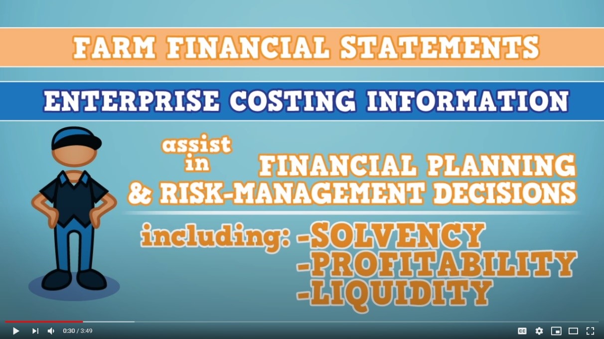
Financial Statements
For an introduction to financial statements watch this video.
Balance Sheet
Most farm businesses are made up of a combination of land, cash, livestock, crops, and machinery (assets), debt (liabilities) and invested equity. The balance sheet summarizes the assets and liabilities for your business. It is like a photograph of these assets (investments and cash) and liabilities (debt) on a given date.
| Assets = liabilities + equity |
Assets: include cash, accounts receivable, inventory (e.g. livestock and crops), automobiles, machinery and equipment, and property (e.g. land and buildings)
Liabilities: include accounts payable, credit cards, mortgages and loans
The balance sheet often reports items as current (less than 12 months), intermediate (1-10 years) or long term (more than 10 years) which includes mortgages and longer-term loans. You may have one business balance sheet and one personal balance sheet for off-farm self-employment.
Tip for reviewing balance sheets:
- Save balance sheets by date and make comparisons at the same time each year
Data to record: Inventories of all commodities on the farm. Many accounting programs will automatically reduce inventory when commodities are sold. If using an excel or paper system remember to reduce commodities on the balance sheet as you sell them. An ongoing record of livestock inventories (total, deaths, missing, sold, purchased, etc.) can help keep your balance sheet current and avoid additional work when the data is needed. Crop or forage inventories can be recorded following harvest or when feed sources are purchased.
When to record it: The month of your year end
Net Worth Statement
Your Net Worth Statement is similar to the balance sheet, evaluating assets and liabilities. Where the balance sheet represents costs (less depreciation), the net worth statement reports fair market value.
| Net worth = fair market value assets – fair market value liabilities |
Comparing Net Worth Statements compiled at the end of each year and over several years can help you measure the progress of your farm business. The net worth statement also helps you judge the ability of the farm operation to pay off current debts and take on additional debt.
Data to record: Start with the balance sheet and adjust every value to the current fair market value of the date selected.
When to record it: When you are going to be using the statement, because current values are used and they change.
Difference between a Balance Sheet and Net Worth Statement
A balance sheet provides the purchased value for assets. These are stable numbers that do not fluctuate from year to year. On the capital asset side, the balance sheet is the cost of the assets less depreciation. The purpose of this information is to provide a more stable valuation that does not fluctuate with the markets. This shows the farm’s ability to produce income. This is what you use for calculating financial ratios (see Level 3 for more information on financial ratios).
A net worth statement uses current fair market values for your assets. Having a list of current fair market values provides greater borrowing power when talking with a banker about a loan because it shows the appreciation of assets and loan carrying capacity.
Making Sense of Farm Equity and Net Worth
Equity is the value of a property in excess of all liabilities against it. In sole proprietorships and partnerships net worth is equivalent to retained earnings (aka shareholder equity). A corporation has multiple sources of equity (shares and retained earnings).
| Equity = assets – liabilities |
Commodity markets, including beef, work in a 10-12-year cycle of highs and lows. During the years with improved profitability, operations can build up farm equity (e.g. land or breeding stock). Building equity when profitability is high helps to mitigate risk when profitability is low.
Data to record: The information needed to review farm equity can be found in the balance sheet.
 Example: Consider two scenarios: in both cases the operations are farmed identically, and the land will be used as a retirement fund. However, not all investments in assets (such as land or equipment) result in building of equity over time.
Scenario 1: An operation where land is owned outright (inherited from the previous generation) and is expected to increase in value over time (providing a retirement fund). During the years when prices are high, income is spent on equipment. During years of negative margins, assets like land and cattle are liquidated. Over time, the new equipment depreciates in value, while the appreciation in land value occurs on fewer total acres. Consequently, equity is reduced over time.
Scenario 2: An operation where land is owned outright (inherited from the previous generation) and is expected to increase in value over time (providing a retirement fund). During the years when prices are high, income is spent on land purchases. Payments are made on an annual basis, including interest. In good years, additional income is spent on paying down loan principles or invested. During years of negative margins, investments may be sold or the land can be used as collateral for a bank loan. Over time, equity is built as new land purchases add to the existing land base; amplifying the appreciation in land value. Consequently, equity is increased over time.
By the time of retirement, the operation in the second scenario will have more assets to work with due to the investment in assets that will increase in value, such as land.
Income Statement
We have just talked about how you may spend your money on assets. Now we will focus on how you generate that cash. A farm income statement is a summary of income and expenses that occurred during a specified accounting period, usually the calendar year. It is a measure of inputs and outputs in dollar values. It also offers a condensed view of the value of what your farm produced for the time period covered and what it cost to produce.
| Net Income = income - expenses |
Most farm managers do a good job of keeping records of income and expenses for the purpose of filing income tax returns. Values from the tax return provide a historical perspective on the income generating capability of the assets. In order to look forward in predicting the financial performance of the farm for the next year one must look at the combination of the balance sheet and income statement together.
The income statement will look different for a cash or accrual accounting system (see table below). Remember that the difference between cash versus accrual accounting is about the timing of when revenue and expenses are recorded (see Cash vs. Accrual Accounting section above).
A cash income statement identifies when expenses are paid and revenue is received, at cost. An accrual income statement gives you the opportunity to see the change in value of inventories (e.g. grain, hay, cattle) and recognize produced inventory.
Income statements (sometimes called a profit and loss statement) can be presented in different ways: with depreciation, without depreciation, with income tax, and without income tax.
Data to record: Collect receipts related to your farm business, remember to ask for receipts when you travel for your farm business.
When to record it: (see Table below) Monthly in conjunction with review of the bank statement.
Example: The property tax for your operation is $1,000 each year. For unforeseen reasons, you need to pay two years’ worth of property tax at the same time. In cash accounting, this payment appears in your records as $2,000. In an accrual accounting system, the expense is recognized as $1,000 in year one and $1,000 in year two; because the payment is for two separate annual payments (with $1,000 recorded as an account payable).
Cash Flow Statement
The cash flow statement is your everyday cheque book accounting which shows money coming in and going out. With the cash flow statement, you can plan your income and expenses over the year.
By having a better understanding of your cash flow over the span of a year you can identify:
- If you may need an operating loan
- When to schedule mortgage or other large payments
- When to schedule capital purchases (i.e. equipment, land, infrastructure, etc.)
Data to record: Most of the information needed to prepare a cash flow statement can be found in combining information from the income statement and balance sheet.
When to record it: (see Table below)
Example: A producer is using cash accounting for tax purposes. He adds a balance sheet to his accounting set up, with stable asset values. He can now use his income statement along with the balance sheet to create a cash flow statement. The balance sheet shows land was purchased (increasing assets) utilizing a bank loan (increasing liabilities). The cash portion of the land purchase shows up as a decrease in cash on the cash flow statement. With this purchase more inventory was produced showing up on the accrual income statement and the balance sheet as having more inventory for sale.
Differences between Income Statement and Cash Flow statement
Terminology matters, but we don’t always correct each other. Imagine you are picking up your city cousin at the airport and on the way home they admire the herd of “cows” in a field. Do you point out that they are actually “steers” or not? A castrated male is significantly different than a reproducing female – but the clarification is not always needed. Accounting, like the beef industry, has its own set of terminology. Sometimes, different names are used for the same financial statements (such as profit and loss statement or income statement). But the differences matter if you are going to be digging into your own farm financials.
An income statement is different from a cash flow statement as shown in the table below and described in the financial statements video above.
- Items in bold and italics denote the differences between using a cash or accrual accounting system. This is about the differences in timing of when sales, other revenue and expenses are accounted for.
- It should be recognized that a cash flow statement is the same regardless of the accounting system used because it is about the cash flowing into and out of a bank account.
- Items in bold only, denote the differences between items that are included in one type of statement but not another.
- This is the farm cash flow, not a household cash flow. You can choose whether T4 wages are included in the cash flow even thought they are not part of the farm. Particularly if they are subsidizing the farm with off-farm income to make loan payments.
Questions about reading financial statements can be directed to your accountant.
Table 4: Differences in data used for cash and accrual Income Statements and Cash Flow Statements
| Income Statement using a Cash accounting system | Income Statement using an Accrual accounting system | Cash Flow Statement |
|
Income
Other Income
|
Income
Other Income
|
Income
Other Income
|
|
Expenses
|
Expenses
|
Expenses
|
Calculating COP
Calculating your cost of production starts with collecting the production and financial records for your operation mentioned in the previous modules. In order to not be overwhelmed, it can be easier to track production information periodically throughout the year.
Tips to help you get started:
- Figure out what your production costs are. You can figure this out by having a conversation with your accountant or using the costs submitted for farm insurance or business risk management programs.
- Determine your costs on a per cow basis. This is calculated by dividing total costs by your ACTUAL number of cows. This takes into account the reproductive efficiency.
- Keep a monthly feed inventory to help determine your feed costs. What was fed? How much? What was the cost?
- Keep track of when you started winter feeding and when cattle were turned out onto pasture.
- Cost of pasture
- Cost of herd health program
- Infrastructure/equipment costs, labour, depreciation (more in-depth enterprise analysis to be covered in Level 3)
Per Unit Cost of Production
 For cow-calf producers, determining the break even price of your calves is one of the first steps you can take towards using records to ultimately improve profitability. The break-even price on weaned calves is known as the cow-calf unit cost of production. Often, cost of production benchmarks are reported as dollars per cow, but having the cost of production is in dollars per lb of calf weaned allows you to develop a risk management plan (such as knowing the level of price insurance to cover costs, if available in your area) and know profitability as soon as the sale price has been set.
However, a cow-calf operation rarely exists as a sole enterprise. If a producer has a cow-calf operation, raises their own replacement heifers, keeps back some calves to background and sell in the spring, and produces their own hay and pasture to graze, they essentially have five enterprises or business lines.
Each of these enterprises has its own cost of production. It is advisable for a producer to separate their costs and revenues into the respective enterprises to determine the cost of production for each. Doing so will enable a producer to see which enterprises are making money and which are losing money.
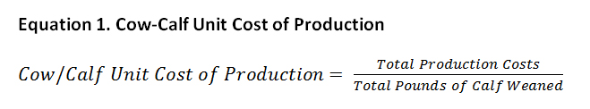
One method of looking at your per unit cost of production or break-even price is by dividing total production costs for the cow herd by the total pounds of calf weaned (see Equation 1 below). As the equation illustrates, a producer’s break-even price can be improved by either: a) reducing production costs, or; b) increasing pounds of calf weaned. Knowing production costs expressed as $/lb of weaned calf allows for direct comparisons with market prices.
A free, Microsoft Excel-based tool was developed by the former Western Beef Development Center, in 2014 for producers to use at home. The Excel tool can be used to enter your own production and financial information, throughout the Excel tool are helpful hints to guide the data entry process. A populated example is also available to show how the data can be entered into the tool.
When to record it: Annually
Example: The following video series from the former Western Beef Development Centre presents more information about the what and the how of determining cost of production: https://youtu.be/u41rVFpZxJs?t=52
Resources to help get you started:
2020 Cost of Production: Pasture https://www.gov.mb.ca/agriculture/farm-management/production-economics/pubs/cop-forage-pasture.pdf
Beef Farmers of Ontario Profitability Calculator: https://www.ontariobeef.com/markets/profitability-calculator.aspx
Rancher’s Return Lite- Cow-Calf and Backgrounding Analysis Tool: https://www1.agric.gov.ab.ca/$Department/softdown.nsf/main?openform&type=RanchersReturnLite&page=information#feed
Western Beef Development Centre: http://westernbeef.org/cowprofits.html
Go Back to Level 1 | Go to Level 3
Feedback
Feedback and questions on the content of this page are welcome. Please e-mail us.