
Level 3
 The Level 3 record keeping resource has been designed to build upon the modules covered in Level 1 and Level 2 The record keeping and benchmarking modules are designed to be used by a wide range of producers and management systems. The purpose of Level 3 is to dig deeper into analysis and application of collected farm data.
On this Page
- Animal Health and Performance
- Forage and Grasslands
- Genetics
- Financial
Animal Health and Performance
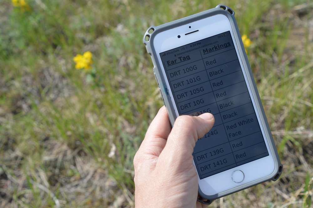
Animal health and performance records can be helpful for making management decisions. Keeping track of your health treatments and performance indicators throughout the year can be useful information to have when evaluating your production goals. Having readily accessible records can also be handy when marketing cattle to prospective buyers.
Sorting Calf/Cow Records Based on Management Groups
A contemporary or management group is a group of animals that are of the same sex, are similar in age, and have been raised in the same management group (same location on the same feed and pasture, at the same time) and if applicable, were weaned and weighed on the same day. Contemporary groups should include as many cattle as can be accurately compared under similar management. For example, if first-calf heifers are given preferential treatment (better feed) prior to weaning their calves, these calves should be designated into a separate contemporary group than the calves from mature cows1.
Sorting animal records based on contemporary groups reduces variability between groups and provides greater ability to make clear comparisons among groups of animals by controlling for management and environmental conditions.
Data to record: for each group, record the individual animal ID, sex, age, location, diet (e.g. creep fed), weights, and other applicable information such as weaning date or whether the offspring is from a first-calver.
When to record it: at sorting, at weaning
Example:
To compare the weaning weights of 50 calves coming off the same pasture on the same day, the calves are grouped based on sex, age, and whether their dam was a first-calf heifer or mature cow. The average weight of the 50 calves as a large group is 604 lbs. By breaking down the groups of calves into contemporary groups, the effect of the dam and sex is more obvious after calculating the pounds gained per day.
| Dam | Sex | Total calves | Average Age (days) | Average Weaning Weight (lbs) | Lbs/day |
| First calvers | Heifers | 3 | 250 | 500 | 2 |
| Bulls | 2 | 250 | 550 | 2.2 | |
| Mature cows | Heifers | 20 | 220 | 600 | 2.7 |
| Bulls | 25 | 220 | 625 | 2.8 |
Calculating 205-day Self Adjusted Weaning Weights
Calculating the 205-day self adjusted weaning weight is one step beyond the comparison of weaning weights at the individual or contemporary group level. To make a fair comparison of calves of various ages and from dams of various ages, calculating a 205-day adjusted weaning weight can give a more accurate picture of both dam and calf performance. By making this adjustment the variability of the calf’s and dam’s ages is removed which provides a better picture of how the calves are performing because the calves are now compared as if they were the same age, and from similarly aged dams.
The Beef Improvement Federation (BIF), an international organization dedicated to standardizing animal performance records across breeds and countries, recommends that weaning weights be standardized to 205 days-of-age and a mature age-of-dam basis. The chart below provides adjustment factors to use when calculating 205-day weights.
Table 1: BIF Standard Adjustment Factors for Weaning Weight
| Age of Dam at Birth of Calf | Male | Female |
| 2 | +60 | +54 |
| 3 | +40 | +36 |
| 4 | +20 | +18 |
| 5-10 | 0 | 0 |
| 11 and older | +20 | +18 |
Data to record: individual ID, sex, birth weight, weaning weight, weaning age, age of dam,
When to record it: collect ID, sex, birth weight, and dam age at birth; collect weaning weight and age at weaning.
Example:
From your records, you have identified achieving higher weaning weights as one of your production goals. From your current calf crop you want to select the heifer calves that will have the best chance of producing calves with higher weaning weights. To do this, calculate the 205-day adjusted weaning weights for the group of heifer calves, and make a decision based on the results.
For example, a 220-day old heifer calf had a weaning weight of 610 lbs and a birth weight of 85 lbs. Her dam was 4 years old at her birth.
To calculate the 205-day adjusted weight:
610 lbs Weaning weight – 85 lb birth weight = 525 lbs
525 lbs ÷ 220 days old = 2.39 lbs/day
2.39 lbs/day X 205 days = 489 lbs + 85 lb birth weight = 574 lbs
Add 18 lbs dam adjustment = 592 lbs adjusted 205-day weight
Example goals:
- Link heifer performance data to their dams for the next calf crop
- Use adjusted weaning weight as a selection criterion when selecting the next group of replacement heifers
Forage and Grasslands
Pasture is a critical resource in the cattle industry. An effective management plan requires realistic production goals, a clear understanding of forage production, effective grazing strategies and timely responses to forage availability and changing environmental conditions.
Identifying Goals
One of the first steps in effective grazing management is to identify the goals for your production system. This includes profitability measures, lifestyle choices, and biological outcomes such as soil health, forage production, ecosystem impacts and animal performance.
Some example goals may include:
- Improving stability of the grazing system by increasing drought preparedness
- Improving health and performance of native pastures
- Improving animal performance by matching forage demand with supply
- Adjusting the number of grazing days according to animal type (cow/calf pairs vs. yearlings)
This list is not exhaustive. Consider your own unique grazing management goals and situation.
Balancing Forage Demand and Supply
The first principle of grazing management is to balance the available livestock demand with forage supply.
Livestock Forage Demand
Livestock forage demand accounts for the nutritional requirements of the animals that will be grazing and consuming the forage. Since animals of differing weights and stages of production have different requirements, this needs to be accounted for.
Animal Unit Equivalents (AUE) and Animal Unit Months (AUMs)
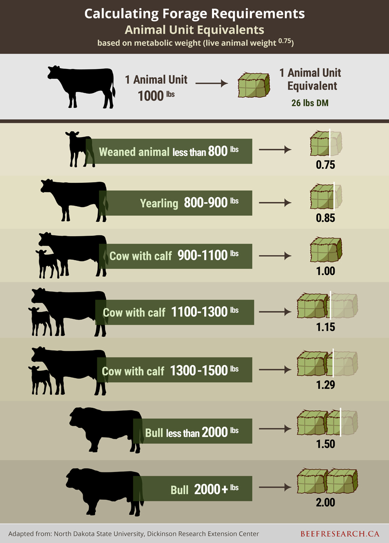
The animal unit (AU) is a standard unit used in calculating the relative grazing impact of different kinds and classes of livestock. One animal unit is defined as a 1000 lb (450 kg) beef cow with or without a nursing calf, with a daily dry matter forage requirement of 26 lb (11.8 kg).
An animal unit month (AUM) is the amount of forage to fulfill metabolic requirements by one animal unit for one month (30 days). One AUM is equal to 780 lbs (355 kg) of dry matter forage.
Because forage requirements change with the size and type of animal, an animal unit equivalent (AUE) is an adjustment to the standard animal unit that takes into account that not all animals weigh 1000 pounds. As a result, the amount of forage dry matter consumed is not always 26 pounds per day.
Data to record:
Type and number of animals: the type of animals that will be grazing such as cow-calf pairs, yearlings, replacements and the number of animals will be required to calculate the grazing demand.
Animal weights: weights will be required to determine what your animal unit equivalents are (1000 lb cows vs. 1500 lb cows).
When to record it: at turn out, and when animals are weighed.
Example:
Typically, beef cows weigh anywhere from 1250 to 1500 pounds. Cows in this weight range can consume between 15 to 30 per cent more forage than the standard 1000-pound cow-calf pair that one Animal Unit Equivalent is based on.
For a group of cow-calf pairs the average weight is 1250 lbs. This means the animal unit equivalent for each pair is 1.15.
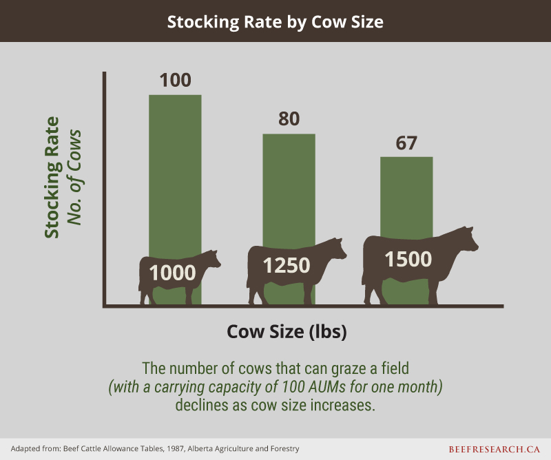
Total forage demand for one month for 100 cows averaging 1000 lbs, is less than that of a herd of 100 cows averaging 1,250 lbs. The number of animals that a pasture can hold (forage supply) will decrease as the size of each animal increases. For the 1250 lb cows, this number decreases from 100 to 80.
Determining the demand from the animal side is only one piece of a successful grazing management plan. To prepare a grazing plan, the supply of forage available for grazing also needs to be determined. Calculating the carrying capacity is one method to measure available forage.
Forage Supply Available
In Level 1, the records for pasture identification, pasture size, grass type, and range health were discussed. This information will be needed to determine the supply of forage available to balance with the demand from grazing animals. By ensuring there is adequate forage available for the number and size of cattle and for the length of time they will be grazing will avoid overstocking or overgrazing the pasture.
Calculating Carrying Capacity
|
*Disclaimer It is important to note that the ideal grazing situation is typically only ideal on paper. There are several factors that are involved in a grazing system therefore it is important to monitor and adjust accordingly. |
When the demand is known, the supply can be managed to meet that demand. Carrying capacity (also known as grazing capacity) is the amount of forage available for grazing animals in a specific pasture or field.
Carrying capacity can be calculated using a variety of techniques. All of them depend on trial and error to some extent and should be monitored and adjusted over time. The carrying capacity for an individual year will vary from the long-term average for the pasture due to the annual environmental conditions, the class of cattle grazing, etc.
In Level 1, the data for pasture identification, pasture size, grass type, and range health were recorded. The BCRC Carrying Capacity Calculator will use this data to determine the available forage supply to meet animal demand.
Forage supply (lbs/acre): The forage supply will be determined in steps 1 and 2 of the carrying capacity calculator. For these steps you will need to have the results from native or tame pasture assessments, which includes estimates for:
- Potential yield of the area (as a %)
- Production from desirable, adapted grass and legumes (as a %)
- Production from weeds or undesirable plants (as a %)
- Fertility program (average, above average, non-existent)
- Precipitation zone (mm/inches)
In step 3 of the carrying capacity calculator, total available forage is calculated using forage supply values, pasture size, and utilization rate.
Utilization rate: The utilization rate determines how much forage is used or lost to grazing, trampling, insects and wildlife. This helps determine how much forage material should be left behind to maintain future production. Utilizing pasture at a rate that exceeds the plant communities' ability to recover can lead to lower forage production and encourage less palatable/productive forage plants to invade the pasture, including weeds. Recommended utilization rates for native pastures vary from 25-50%. For tame pastures, recommended utilization rates range from 50-75% depending on fertility.
The BCRC Carrying Capacity Calculator provides two methods: 1) estimates based on provincial guides and 2) field-based sampling.
Producers can use the Method 1 calculator if they wish to calculate an estimate of carrying capacity based on available provincial forage production guides. Using Method 1 is easy and works best when the pasture condition (or range health) is similar throughout the field and the forage plant community (or range type) is uniform.
Producers can use Method 2 if they plan on clipping, drying, and weighing samples collected from their pasture. Field-based sampling provides greater accuracy but requires more hands-on work. Producers may choose field-based sampling if provincial guides are unavailable for their region or if pasture types or conditions vary within their field. Forage production varies each year, so the Method 2 approach should include multiple years of sampling to estimate the long-term productivity of the pasture.
The following BCRC webinar provides step by step instructions on how to use both methods of the Carrying Capacity Calculator.
Data to record:
See Level 1, for the records for pasture identification, pasture size, grass type, and range health.
When to record it: prior to turn out
Example:
The following video provides greater detail about using the carrying capacity calculator to determine total forage available, the corresponding number of animals that can graze the pasture, and the number of grazing days available.
This process of completing an inventory and evaluating resources is critical to developing and implementing a successful grazing system. The Pasture Planner: A Guide to Developing Your Grazing System provides an excellent resource to assist producers with planning, development and/or modification of their grazing system. It includes a number of worksheets and templates useful in the inventory and planning process.
Prepare a Grazing Plan
When the carrying capacity of various pastures are known, a grazing plan can start to take shape. In addition to this information, conducting a more in-depth inventory of resources is essential. Regardless of the pasture type, focusing on a few key principles can help maintain forage productivity, ensure stand longevity, sustain a healthy plant community, conserve water, and protect soils. In addition to balancing supply and demand, here are some points to consider:
- What is the relative yield and periods of growth for individual pastures throughout the grazing season?
- When is the best time to provide periods of rest and recovery for each pasture?
- Distribute grazing pressure across the pasture. When left on their own, cattle will prefer to graze moist, productive areas of a pasture and avoid dry hilltops where the forage quality may be lower.
- Which pastures will be needed and are best suited for a specific time period during the grazing season? Avoid grazing during sensitive times. Grazing too early can set a pasture back for the whole season.
- What physical infrastructure (e.g. fencing, water) is available or needed?
There are many different types of grazing systems promoted by groups and individual producers, including, but not limited to, rest-rotation, AMP (adaptive multi-paddock), intensive, or strip grazing. While each system has its own benefits and drawbacks, almost all systems factor in the key principles of grazing management.
Once a grazing plan has been implemented, it will be crucial to monitor and make changes to the plan as the grazing season progresses. Challenges such as drought, may require changes to stocking rates, adjusting rest periods, or providing alternative feed sources if needed. Flexibility is a key component of successful grazing management.
Genetics
In Level 2, identifying your operation’s breeding goals and individual animal identification was discussed. To identify bulls with better calf performance, start by reflecting on what your goals are, and which traits will help you achieve your goals.
Identifying Bulls that Support Your Goals
Once traits have been identified that support your goals, you can compare the performance of calves sired by each bull for these traits. For example, comparing the average weaning weights of live calves sired by all bulls can be used to identify the bull(s) siring calves with higher weaning weights. This provides valuable information when making culling and breeding decisions.
Bull selection is one of the most important decisions for cow-calf producers, with implications for short- and long-term profitability of the operation. The choice of bull can be immediately seen in the next calf crop. If the operation retains heifers and/or bulls, the genetics in the selected bull will be passed down to subsequent generations. Introducing new genetics is a permanent change to the herd, compared to the relatively temporary nature of many feeding management practices. As such, bull selection can be seen as a long-term investment into the operation and should be viewed as an opportunity to make significant genetic improvements.
After the initial investment of purchasing a herd sire, the bull will only provide a return on this investment if he is siring calves. Parentage testing using DNA sampling, particularly on multi-sire pastures, can indicate whether a bull is siring calves as expected. Identifying the progeny of each bull can also provide an opportunity to determine whether a particular bull is:
- Siring calves with traits that support your production goals
- Consistently producing calves with undesirable traits (e.g. poor conformation, calving ease, etc.)
- Not siring as many calves as expected.
The following webinar includes more details about DNA testing in commercial herds with multi sire pastures.
For more information about bull selection, review the Bull Selection series.
Calving Ease Data
Calving ease is a key trait that influences profitability. It is estimated the majority of calf death loss is a result of difficult delivery (dystocia). Dystocia can be caused by a large pre-natal calf, small pelvic area of the dam, lack of sufficient uterine contractions, insufficient dilation of the cervix, or mispositioned calf prior to birth2.
Dystocia results in higher labor costs, decreased calf survival, and delayed rebreeding for the cow, resulting in younger calves at weaning the following year. Issues with dystocia within the herd can be addressed by keeping calving ease records.
Calving ease can be scored using the scores listed in Table 1.
| Table 1: Beef Improvement Federation calving ease scoring guidelines | |
| Score | Description |
| 1 | No difficulty, no assistance required |
| 2 | Minor difficulty, some assistance |
| 3 | Major difficulty, usually mechanical assistance |
| 4 | Caesarian section or other surgery |
| 5 | Abnormal presentation |
Cows that calve between regular checks can be assumed to have calved without assistance even if the calving was not observed. A score of 1 should be reported for these. All calvings should receive a score even if the calf is born dead. These scores may then be used when making culling decisions, particularly if dystocia has been an issue.
Similar to adjusted weaning weights, calving ease comparisons should be made according to contemporary or management group2. Calving ease EPDs are produced from calving difficulty scores and birth weight observations.
The Beef Improvement Federation (BIF) suggests that birth weights alone should not be used as selection criteria and to use calving ease information, if available, instead when making culling or breeding decisions.
Calf birth weight is an indicator trait for calving difficulty. If calving difficulty is a problem in the herd, and calving ease EPDs are not available, selection of breeding animals for lighter birth weight may be an effective strategy to improve direct calving ease. However, selecting for a single trait such as lighter birth weight or shorter gestation intervals may reduce calf viability and growth rate from birth to maturity3.
For seedstock breeders that intend to sell bulls or seedstock females, birth weights must be measured accurately prior to submitting to the breed association for EPD calculation. Accurate birth weights should be measured using a scale. Visual assessment or taping is not considered an accurate measurement.
Data to record: birth weight, calving ease score
When to record it: at birth
Example:
During the morning calf check, three live calves were found. The record for each calf is given a calving ease score of 1 because the calves were all born unassisted.
At culling, your records indicate that most of the herd received a calving ease score of 2 or less. Cows that received a score of 3 or higher are moved into the cull pen.
Post Weaning Gain and Yearling Weight
In Level 1, the collection and use of weaning weight records was discussed. For operations that retain calf ownership or those that are raising replacement heifers, they may consider collecting post weaning gain and/or yearling weights.
Post Weaning Gain
 Higher growth rates can mean fewer days on feed and lower input costs to reach market weight. Post weaning gain on animals with retained ownership may be linked to sire and dam performance, which can assist with making culling decisions. As with birth and weaning weights, post weaning gains should be taken using an accurate livestock scale.
Data to record: body weight
When to record it: when received from feedlot or after on-farm weigh-in
Example:
The average weaning weight for a group of feeder calves was 550 lbs. After the second weight collection, the group averaged 3 lbs of gain per day. Weights were also given for individual animals according to their CCIA tag number. Sorting the weight data from high to low revealed that all of lighter animals came from the same sire, suggesting the bull may need to be replaced.
Yearling Weight
For replacement heifers, yearling weight records can provide valuable information about the potential of the heifer as a breeding female. It has been suggested that heifers that have reached one year of age should be approximately 55-65% of their expected mature weight5. This guideline is to ensure that yearling heifers will reach sexual maturity prior to the breeding season. This also allows heifers to be bred prior to the mature cow herd and will give heifers enough time to recover from the first calving to rebreed for her second calf.
It should be noted that selecting replacement heifers to produce calves with higher yearling weights can result in larger cows. This needs to be taken into consideration to account for the environment these females will have to survive in since larger cows will need more feed.
Data to record: 365-day weight
When to record it: 160 days after weaning weight or when average group age is between 320 and 410 days.
Example:
A group of heifers has reached an average age of 360 days. Individual weights are recorded to the nearest pound. The average for the group of heifers is 800 lbs and the average weight of the mature cow herd is 1600 lbs.
800 lbs / 1600 lbs x 100% = 50% of mature cow weight
The group of heifers was divided into two groups, calves sired by Bull A or Bull B. The heifers from Bull A have an average weight of 900 lbs and Bull B’s heifers have an average of 750 pounds.
Bull A sired: 900 lbs / 1600 lbs x 100% = 56%
Bull B sired: 650 lbs / 1600 lbs x 100% = 47%
The breeding season is still 60 days away. If the heifers are gaining 2 lbs per day on average, that gives each group an opportunity to gain 120 lbs prior to breeding. This would bring each group to:
Bull A sired: 1020 lbs/1600 lbs x 100% = 64%
Bull B sired: 770 lbs/ 1600 lbs X 100% = 48%
Comparing the heifers by sire can identify the females with the greatest potential to pass growth traits onto her offspring and identify the bulls with better replacement heifer performance.
Financial
In agriculture there are many areas of risk and uncertainty. Sectors with tight margins, such as the beef sector, can greatly benefit from having a better understanding of their operation’s finances. Understanding strengths and weaknesses is one way to reduce the stress that comes with uncertainty and provide financial resiliency to help an operation adapt to challenges.
Farms often have to make quick financial decisions; impacted by weather or other outside variables. Knowing one’s financial ratios gives options as they can represent possibilities and flexibility for the operation in how they respond. Farm businesses should have a good working relationship with their financial institutions, whether they are leveraged or not, as those quick decisions can be smoother with an existing creditor relationship.
Financial ratios can be used to analyze an operation over time. Financial ratios do not provide the answers as to why a business is performing well or underperforming, although they can help point out the areas to examine in order to ask the right questions about the business. They can help identify an operation’s areas of financial risk (stress); and assist in making decisions that affect these numbers. Remember, these ratios represent a point in time and will change depending on the year (e.g. markets, prices of inputs and outputs).
In addition to comparing a business’ historical performance, there are general guidelines that can be used to see how that business compares to an industry ratio range provided (see Table 2). It should be noted that financial ratios will vary by sector and industry. Some ratios are less effective for comparing operations of different sizes.
Table 2. Farm Financial Ratios
| Liquidity | Healthy | Medium | Caution |
| Current Ratio | Greater than 1.5 | 1.0 - 1.5 | Less than 1.0 |
| Working Capital | Greater than 30% | Greater than 30% | Less than 30% |
| Solvency | |||
| Debt to Asset Ratio | Less than 30% | 30% - 60% | Greater than 60% |
| Equity to Asset Ratio | Greater than 70% | 40% - 70% | Less than 40% |
| Debt to Equity Ratio | Less than 0.3 | 0.3 – 1.0 | Greater than 1 |
| Profitability* | |||
| Return on Assets (ROA) | Greater than 0.05 | 0 - 0.05 | Less than 0 |
| Return on Equity (ROE) | N/A | N/A | N/A |
| Operating Profit Margin Ratio | N/A | N/A | N/A |
| Net Farm Income | N/A | N/A | N/A |
| Repayment Capacity | |||
| Debt Payout Ratio | Greater than 135% | 110% - 135% | Less than 110% |
| Debt Service Coverage Ratio | Greater than 150% | 130% - 150% | Less than 130% |
| Financial Efficiency | |||
| Asset Turnover Ratio | Greater than 0.15 | 0.02 – 0.15 | Less than 0.02 |
| Operating Expense Ratio | Less than 70% | 70% - 95% | Greater than 95% |
*There is no recommended metric for profitability as this will vary depending on farm size.
Every operation will be different, some will have short-term debt, others will have long-term debt. Some will be leveraged with a bank more heavily while others utilize internal equity. These choices are as varied as the types of operations found from coast to coast. It should be noted that having a single ratio in the red is not necessarily bad. You cannot look at a single ratio and determine the overall health of a business or farming operation. Multiple ratios must be used along with other information to determine the total and overall economic health of a farming operation and business.
Start by completing a balance sheet and income statement every year-end. As mentioned in Level 2, the balance sheet identifies your business assets, liabilities, and equity. Once these financial statements are completed, there are several financial management measurements that can be calculated. These can be calculated with both cash and accrual statements, whatever you are using.
Liquidity
Taking on more debt to finance the purchase of assets allows a business to expand and grow. Paying off the debt is done with the additional revenues generated by properly deploying these assets. Reducing debt or seeing assets gain value over time are two ways to build equity or net worth. However, financing a large portion of the business growth through debt also exposes a business to financial risk7. Monitoring financial ratios around liquidity and solvency can inform you about how much financial risk the operation has taken on.
Liquidity addresses an operation’s ability to meet short-term debts; while solvency addresses an operation’s ability to meet long-term debts. They are used both independently and together.
Current Ratio
|
Current Ratio = Current Assets / Current Liabilities |
|
Industry Ratio Range The ratio is expected to be more than 1. A ratio > 1.5 is low risk, 1.0-1.5 is medium risk, and < 1.0 is high risk. For the cow/calf sector 1.3 is considered healthy and for the feeder sector 1.5 is considered healthy. |
The Current Ratio (usually expressed as XX:1) measures a business' ability to meet financial obligations as they come due in the next 12 months, without disrupting normal operations. It answers the question whether the operation can pay the current portion of debt owing at a given point in time.
A current ratio less than 1.0 means that a farm lacks the current assets to cover short-term liabilities. A current ratio higher than 1 is healthy. If an operation’s current ratio is too high, it may not be using cash as efficiently as possible. A current ratio of 1 to 1.5 indicates a farm is technically liquid, but it could be exposed to financial challenges if market conditions worsen. This is medium risk.
Data to use: Financial ratios can be calculated by pulling numbers from the balance sheet and income statement. The balance sheet often reports assets and liabilities as current (less than 12 months), intermediate (1-10 years) and long term (more than 10 years) which includes land, buildings, mortgages, and longer-term loans. Intermediate is frequently included with long-term.
Quick Ratio or Acid Test
|
Quick Ratio = Cash Equivalents / Current Liabilities |
The Quick Ratio is a measure of the proportion of cash (or cash equivalents) to current liabilities. Unlike the current ratio, the quick ratio does not include inventories and assets which disrupt normal business operations when converted to cash.
The Quick Ratio is important as it shows if producers can pay off their current liabilities (over the next 12 months) without selling breeding cattle, yearlings, hay, or other commodities that will be produced over the next twelve months.
Working Capital
|
Working Capital = (Current Assets - Current Liabilities) / Annual Expenses |
|
A rough Rule of Thumb is an operation should have a minimum of about 30% of their annual expenses available as working capital |
Working capital is a theoretical measure of the amount of funds available to purchase inputs and inventory items after the sale of current assets and payment of all current liabilities. A ratio of 0.5 means that one has enough working capital on hand to cover approximately 6 months’ worth of expenses.
If working capital is the first line of defence in paying short-term debt, not having access to capital can force an operation into secondary means of repayment (refinancing of debt) or possibly even selling assets9. The amount of working capital considered adequate must be related to the size of the farm business.
Solvency
Solvency ratios include financial obligations in both the long and short term and measures an operation’s ability to meet those obligations. Solvency ratios assess long-term economic health by evaluating repayment ability for long-term debt and interest on that debt.
Debt to Asset Ratio
|
Debt to Asset ratio = Total Liabilities / Total Assets |
The Debt to Asset Ratio shows the portion of total assets financed through debt. This ratio is a measure of the extent of creditor financing used by the business. The higher the value of the ratio, the higher the financial risk. A lower debt to asset ratio brings flexibility to an operation if it must withstand challenges or be able to seize opportunities quickly (e.g. expansion, diversification).
It can be calculated by using either the cost or market value approach to value assets. The ratio is most meaningful for comparing between farms when market value is used. But due to market fluctuations, the cost approach is most meaningful for year over year comparisons on the same farm.
Equity to Asset Ratio
|
Equity to Asset Ratio = Total Equity / Total Assets |
The Equity to Asset Ratio is a measure of the extent of leverage being used by the business. It considers the proportion of total assets paid by the owners’ equity versus those financed by creditors. The higher the ratio means more total capital has been supplied by the owners, and less by creditors and, in most cases, the business is more solvent, and better equipped to pay its debts.
Debt to Equity Ratio
|
Debt to Equity Ratio = Total Liabilities / Total Equity |
|
Rule of Thumb for debt to equity ratios, anything above 1 is considered to be higher risk. |
The Debt to Equity Ratio indicates the ability of equity to cover all outstanding debt which includes both short term and long-term obligations. A low debt-to-equity ratio provides flexibility to extend terms on existing debt when profits and repayment capacity are tighter and to borrow more money if an opportunity arises12. In contrast, the higher the ratio, the more total capital has been supplied by the creditors and less by the owners.
These ratios will vary depending upon management and efficiencies of the operation. Feeding operations typically are more leveraged with a higher proportion of debt in current liabilities to finance feeder cattle.
Profitability
A farm business has three ways to increase profits — by increasing the value per unit sold, decreasing the cost per unit produced or increasing the volume produced.
Profitability measures that are universally accepted for their value to management include: return on assets, return on equity, and operating profit margin. They measure the extent to which a business generates net income or profit from the use of its resources. Technically, they are efficiency metrics that measure the relationship between an output, in this case net farm income from operations, and an input.7 However, when evaluating the strength of a loan request, profitability measures can create distracting noise, which is not helpful in a lending discussion.
Return on Assets (ROA)
|
Return on Assets = Income/ Total Assets |
|
Industry Ratio Range Expected to be larger than zero: 0.05-0.1 is a healthy range for beef production. |
The Return on Assets is used as an overall index of profitability. Income is calculated after owner withdrawal for unpaid labour and management have been removed but before taxes and interest have been paid. Removing unpaid labour and management prevents the result from being under- or over-stated. Taxes and interest are not considered because ROA measures the return to all capital, both debt and equity.
The Return on Assets may seem low when compared to non-farm investments such as stocks and bonds. It should be recognized that neither realized nor unrealized gains on farm real estate and other assets are included as income.
The value of the ratio can vary with the structural characteristics of the farm business, especially with the proportion of owned land (or other assets) used in the farming operation. A higher ratio is an indication of greater profits and ability to leverage assets to create a profit.
Return on Equity (ROE)
|
Return on Equity = Income / Total Equity |
The Return on Equity is used as an overall index of profitability. Income is calculated after interest, owner withdrawal for unpaid labour and management have been removed, but before taxes. Deferred taxes should be included in the total equity calculation.
Caution should be used when interpreting this ratio. A high ratio, normally associated with a profitable farm business, may also indicate an undercapitalized or highly leveraged farm business. A low ratio, which normally indicates an unprofitable farm business, may also indicate a more conservative, high equity farm business. This measure, like many of the other ratios, should be used in conjunction with other ratios when analyzing a farm business.
Operating Profit Margin Ratio
|
Operating Profit Margin Ratio = Income - owner withdrawal for unpaid labour and management / Revenues |
This ratio measures profitability in terms of return per dollar of revenue. Each farm will have a made a decision about paid labour, unpaid labour and owner withdrawal that will show up on the balance sheet and income statements used to calculate these ratios. The Operating Profit Margin Ratio shows what the owner is withdrawing to live on if anything.
Net Income
|
Net Income (before income tax) = Total Revenue – Total Expenses (before income tax) |
Net Income is the return to the producer for unpaid labour, management, and owner equity. The measure is a dollar amount (which may be positive or negative); therefore, it is difficult to compare across farm businesses. You may find it easier to compare from year to year by making an accrual adjustment (If the income statement is prepared using cash accounting, then both beginning and ending balance sheets are needed to make the necessary adjustments for changes in inventories, accounts receivable, accounts payable, prepaid expenses and accrued expenses).
Repayment Capacity
The two main measures to assess an operation’s debt repayment capacity are its balance sheet and cash flow measures. By analyzing key metrics from the balance sheet and cash flow statements, creditors determine the amount of sustainable debt a company can handle.
Debt Payout Ratio
|
Debt Payout Ratio = Total Liabilities / Net Income |
The Debt Payout Ratio shows how many years are required to pay all the debts through net returns. A lower number indicates it will take the operator less time to pay down debt. Remember that land mortgages are typically amortized over 20, 25, or 30 years.
This number will reflect where an operation is in its lifespan; a new operation will have more debt with a higher ratio and a mature operation with a retirement plan will have a lower ratio. Operations in the process of succession planning will vary based on the stage and situation (e.g. if they are expanding).
Data to use: Everything up to this point can be calculated by pulling numbers from the balance sheet and income statement. For this ratio, start by calculating your Net Income, as shown in the Profitability section.
Debt Service Coverage Ratio (DSCR)
|
Debt Service Coverage Ratio = Income / Debt Service |
The Debt Service Coverage Ratio (DSCR) measures an operation’s cash flow available to service debt. This is used by banks to assess the customers’ capacity to repay their existing long-term loans and take on new long-term loans.
|
Industry Benchmark The average Debt Service Coverage for the beef Industry is > 1.30:1 or 130% |
“Income” is defined as net cash income (farm revenues after taxes minus operating expenses before interest payments) plus other income and off-farm income. NOTE: elsewhere income is only on-farm income and excludes off-farm income, this is the exception. “Debt service” includes the current portion of long-term debt (loan principal due in the next twelve months or current portion of lease payments, for example) plus interest.
A DSCR of 1.5 indicates an operation has 1.5 times more cash available to pay current debt obligations than the total amount owing. A ratio below 1 indicates an inability to rely on net cash income and off-farm income to service debt.
If a DSCR is too low, a farm may find it hard to make payments on what is owed using only revenues. A very high DSC may not be optimal either. While it can reflect an operation that does not need debt to generate revenue, it may also point to one that is not exploiting market opportunities.
Scenarios can be conducted to assess how a reduction in revenue, or increase in production costs, or variable expenses will affect the debt service coverage ratio.
Financial Efficiency
Financial efficiency is all about getting more output from the same resources or getting the same output from fewer resources. There are efficiency ratios used to measure either production or financial efficiency, or a combination of both.
Asset Turnover Ratio
|
Asset Turnover Ratio = Total Revenue / Total Assets |
|
Industry Ratio Range There is no hard benchmark for this. A value of 0.15 or higher can be considered good. |
All farms use the assets they have in land, buildings, equipment, and breeding livestock to generate sales, or revenue. The Asset Turnover Ratio is calculated by dividing total revenue by total assets. It is a measure of the extent to which a business uses its assets to generate revenue. The higher the ratio, the better the assets are being used to generate revenue.
The asset turnover ratio shows how much revenue is produced per one dollar of asset. For the beef sector, a value of 0.15 is healthy (that is 15 cents for every dollar of asset).
Operating Expense Ratio
|
Operating Expense Ratio = Operating Expenses / Total Revenue |
|
Industry Ratio Range Expected to be less than 1 to have sufficient cash on hand. Can be around the 70% for cow/calf producers and 95% for feedlot operations depending upon location and management. |
The Operating Expense Ratio measures an operation’s variable (aka operating) costs relative to total revenue. An operating expense ratio of 0.7 indicates an operation spends 70% of its revenues on variable expenses.
If the ratio is too high, a farm may have higher expenses than it can be expected to cover with revenue. This could possibly expose a producer to financial challenges if market conditions worsen, and an overly high operating expense ratio also reduces the income available to cover fixed costs or build equity8.
Data to use: From the income statement use the variable (aka operating) expenses. Variable expenses include daily operational expenses (labour, feed, crop protection, fuel, maintenance, insurance, repairs, and service provider fees, for example). Loan payments, depreciation, and capital improvements are excluded from operating expenses8.
Example
Example farms are provided utilizing the sample Financial Statements (see the linked Balance Sheet and Income Statement for details). The ratios presented in Table 3 are calculated from these financial statements.
Table 3. Sample Farm Financial Ratios
| Financial Ratios | Farm ABC | Farm MNO | Farm XYZ |
| Current Ratio = Current Assets/Current Liabilities | 2.78 | 0.93 | 1.72 |
| Quick Ratio = Cash Equivalents / Current Liabilities | 0.07 | 0.23 | 0.07 |
| Working Capital = (Current Assets - Current Liabilities) / annual expenses | 30% | -4% | 21% |
| Solvency | |||
| Debt to Asset Ratio = Total Liabilities/Total Assets | 0.24 | 0.59 | 0.31 |
| Equity to Asset Ratio = Total Equity / Total Assets | 0.76 | 0.41 | 0.69 |
| Debt to Equity Ratio = Total Debt / Total Equity | 0.31 | 1.41 | 0.45 |
| Profitability | |||
| Return on Assets = Income / Total Assets | 0.36 | 0.52 | 0.11 |
| Return on Equity = Income/ Total Equity | 0.48 | 1.26 | 0.16 |
| Operating Profit Margin Ratio = Income - owner withdrawal for unpaid labour and management / Revenues | 0.94 | 1.00 | 0.98 |
| Net Income (before income tax) = Total Revenue - Total expenses (before income tax) | $197,100 | $91,811 | -$39,097 |
| Repayment Capacity | |||
| Debt Payout Ratio = Total Liabilities / Net Income | 3.04 | 8.39 | -19.68 |
| Debt Service Coverage Ratio | 94% | 37% | 17% |
| Financial Efficiency | |||
| Asset Turnover Ratio = Total Revenue / Total Assets | 0.36 | 0.52 | 0.11 |
| Operating Expense Ratio = Operating Expenses / Total Revenue | 0.68 | 0.04 | 0.59 |
Farm ABC has chosen to put cash into inventory, reflected in the large operating expenses as a percentage of total expenses. It is an indication they are purchasing all their feed and have large animal purchases.
Farm MNO has chosen to keep cash on hand versus investing in long-term assets. The current year has more liabilities making it a year to pay off loans, but these loans could be what is making them appear profitable. This means they will have to monitor cash flow carefully throughout the year. While working capital is negative, net income is positive and they have cash on hand. This is why it is important to look at multiple financial indicators and any single indicator in isolation. This also means that next year they could be significantly improved. They are heavily leveraged, and currently have a small amount of equity so they have a smaller return on equity.
Farm XYZ is a farm with land mortgages showing up in the long-term debt. The majority of the land is rented out, but they are farming a portion of the land. However, this was a poor production year as cash and inventories are low. The debt payout ratio is negative while the debt service coverage ratio indicates that off-farm income is being used to make debt service payments.
Gross Margin Ratio
|
Gross Margin Ratio = Income from enterprise X / Variable expenses from enterprise X |
Gross Margins provide a method of comparing the performance of each enterprise. A gross margin refers to the total income derived from an enterprise less the variable costs incurred in the enterprise.
|
Enterprise: An enterprise can be defined as the commodity that is produced, the method that is used or by the activity being performed. For example, beef and hay production are two different commodities. Beef production can be sub-divided based on the stage of growth of cattle, production methods or other activities (e.g. replacement heifers, backgrounders, animals in a certified program with specific production parameters). |
Variable expenses (or operating expenses) include feed, crop protection, fuel, maintenance, insurance, repairs, and service provider fees. Loan payments, depreciation, and capital improvements are excluded from operating expenses8.
Producers must choose which enterprise each of these variable expenses apply to. The benefit of the gross margin ratio is the fact that you do not have to allocate fixed/overhead costs to each enterprise. These fixed costs are assumed to be part of the operation and gross margin ratios help find which enterprise will contribute the most to covering their costs. However, when an operation has fixed costs that are strongly associated with a single enterprise the gross margin analysis can be misleading. Therefore, capital and labour which are excluded from the gross margin ratios need to be taken into consideration prior to making concrete decisions.
Data to use: Variable costs allocated to each enterprise and income generated from each enterprise.
Scenario: Farm A is considering hiring a custom silage crew, instead of haying with owned equipment. The decision must consider that additional cash expenses will be incurred with custom silage; while it will reduce labour requirements. At the same time, the farm will continue to have the cost of owning the haying equipment.
Farm B is considering using a community pasture when they have deeded land to pay and utilize. They are prioritizing winter feed production on their deeded land. The decision must consider the additional cost of community pasture fees and how expensive that makes the winter feed production.
Farm C is considering buying more cattle to utilize all of their own land and available community pasture for summer grazing. This would mean they would have to buy 100% of their winter feed. If they do not buy their winter feed, they would have to sell their cattle herd. The decision must consider the additional cost of the community pasture and purchasing winter feed with the increase in revenue from a larger cattle herd.
Farm D is considering selling some of their cattle while utilizing the community pasture for their summer grazing. They would use their own equipment and owned land to put up winter feed so that they do not have to buy any winter feed (it would be 100% homegrown). The decision must consider labour availability to grow 100% of their winter feed and understanding that the short-term decision to sell cattle will result in less income next year.
Feedback
Feedback and questions on the content of this page are welcome. Please e-mail us.
Version 1.0 September 2020